> ## Documentation Index
> Fetch the complete documentation index at: https://docs.upsonic.ai/llms.txt
> Use this file to discover all available pages before exploring further.
# Applied Scientist
> Autonomous agent that benchmarks a new method against your existing Jupyter notebook — from a paper, repo, Kaggle link, or a free-form idea.
## What is Applied Scientist
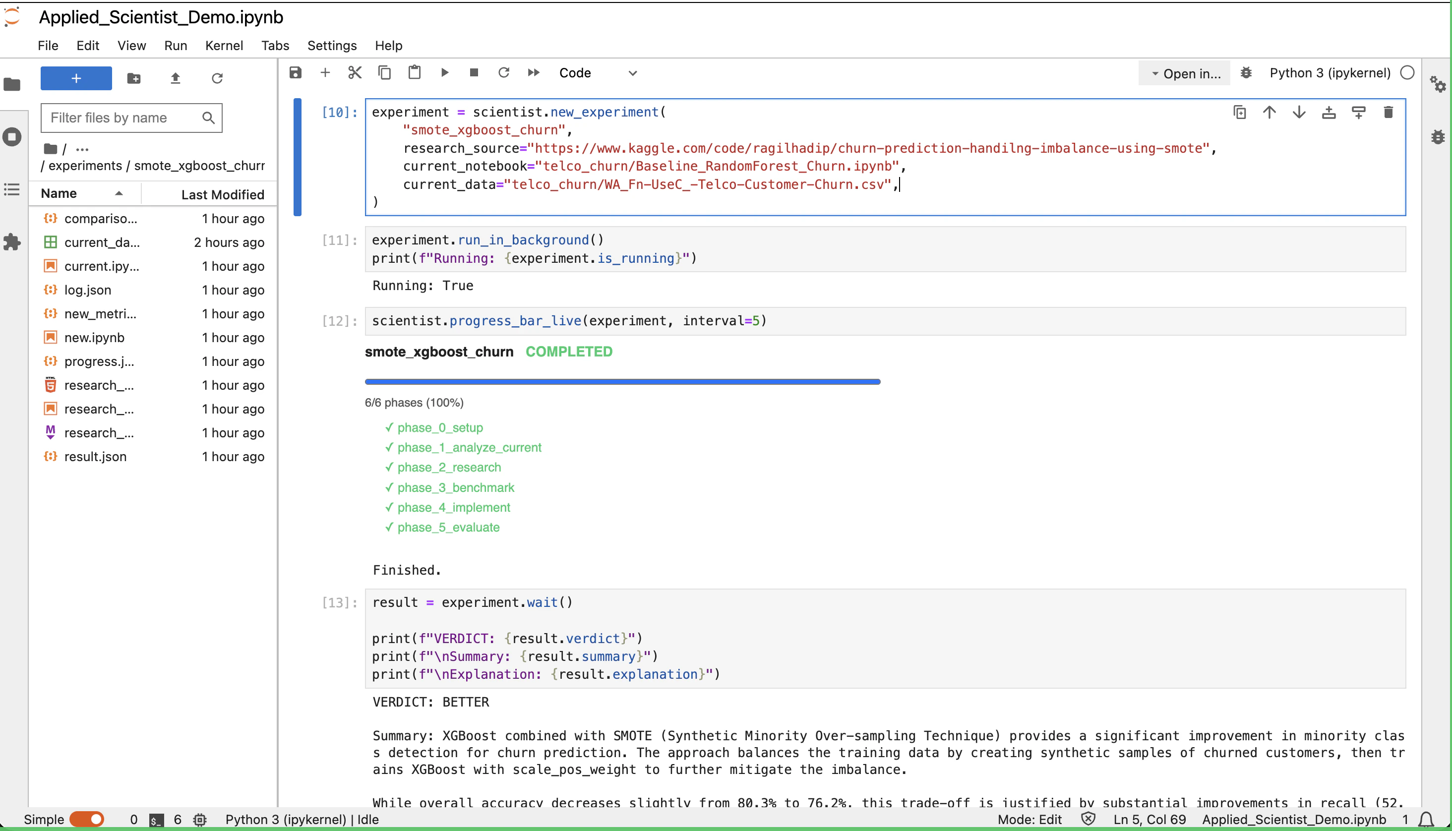
Applied Scientist is an autonomous agent that runs inside Jupyter. You hand it your **baseline notebook** and a **research source** (PDF, web URL, Kaggle link, GitHub/GitLab repo, or a plain-text idea), and it does the work a researcher would do by hand: read it, run your baseline, implement the new method, and produce a structured comparison.
You supply the inputs, launch the run, and read the result.
 ## How It Works
A run moves through six fixed phases. Each phase has one job and hands off to the next.
Creates an isolated workspace and copies your notebook, data, and research source into it. The original files are never touched.
Reads your baseline notebook and documents the model, preprocessing, hyperparameters, and the metrics it reports.
Digests the research source: what the method does, what it improves, its requirements, and whether it's compatible with your data.
Locks in the metrics and baseline values that both sides will be measured on. Missing baseline metrics are flagged so the new run computes them too.
Writes a new notebook implementing the method, using the same data, split, and seed as the baseline. Runs it end-to-end.
Compares both runs and issues a verdict — `BETTER`, `WORSE`, `INCONCLUSIVE`, or `FAILED` — with concrete reasoning recorded to disk.
## Cursor & Claude Code vs Upsonic Prebuilt Autonomous Agents
A question we hear a lot: *why use this instead of just doing the same thing in Cursor or Claude Code?* The short answer is that those are general coding copilots, and Applied Scientist is a purpose-built experiment runner. The table below shows where the two approaches diverge.
| Dimension | Cursor & Claude Code | Upsonic Applied Scientist |
| ----------------- | --------------------------------------------------- | ------------------------------------------------------------------------- |
| Workspace | Runs in your working repo, shared with your editor | Fully isolated workspace folder per experiment |
| Output | Free-form chat and file edits | Structured `ExperimentResult` (verdict, comparison table, metrics) |
| Workflow | Assembled case by case in the chat | Pre-tested, well-designed pipeline |
| Environment | Outside the notebook | Runs directly inside Jupyter |
| Progress tracking | Scroll through chat transcript to guess where it is | Live progress bar driven by `progress.json`, plus `last_logs(n)` timeline |
## Install
```python theme={null}
!pip install upsonic
```
```python theme={null}
import os
os.environ["ANTHROPIC_API_KEY"] = "sk-ant-..."
```
## Requirements
You only need two things on disk.
A working `.ipynb` that trains your baseline model end-to-end. This is the reference every comparison is made against.
Anything describing the method to try: PDF, Markdown/HTML, web URL, arXiv link, GitHub/GitLab/Bitbucket repo, Kaggle notebook or dataset page, or a free-form idea as plain text.
`current_data` is optional. Omit it and the agent reads your notebook to find the data-loading cells itself.
## Running an Experiment
The example below is the demo shipped with Upsonic: a Random Forest baseline for telco customer churn, benchmarked against a Kaggle notebook that uses **SMOTE + XGBoost** to handle class imbalance.
### 1. Create the agent
```python theme={null}
from upsonic.prebuilt import AppliedScientist
scientist = AppliedScientist(
model="anthropic/claude-haiku-4-5",
workspace="./autonomous_workspace",
)
```
`workspace` is the root directory the agent is allowed to work in. Every experiment lives in its own folder inside it.
### 2. Define the experiment
```python theme={null}
experiment = scientist.new_experiment(
"smote_xgboost_churn",
research_source="https://www.kaggle.com/code/ragilhadip/churn-prediction-handilng-imbalance-using-smote",
current_notebook="telco_churn/Baseline_RandomForest_Churn.ipynb",
current_data="telco_churn/WA_Fn-UseC_-Telco-Customer-Churn.csv",
)
```
`research_source` is polymorphic — pass any of these and the agent figures out how to materialize it:
* **Local files** — PDF, Markdown, HTML, `.ipynb`, plain text
* **Web URLs** — blog posts, arXiv pages, documentation
* **Code hosts** — GitHub, GitLab, or Bitbucket repository URLs
* **Kaggle** — notebook or dataset pages
* **Free-form idea** — a plain string describing what to try
| Parameter | Purpose |
| ----------------------- | --------------------------------------------------------------------------------------------- |
| `name` (positional) | Folder name and registry key |
| `research_source` | Anything from the list above |
| `current_notebook` | Path to your baseline notebook |
| `current_data` | *Optional.* Data path or a short loader description. Inferred from the notebook when omitted. |
| `experiments_directory` | *Optional.* Defaults to `./experiments` inside the workspace. |
### 3. Run and watch
`run_in_background()` starts the run in a daemon thread and returns immediately.
```python theme={null}
experiment.run_in_background()
scientist.progress_bar_live(experiment, interval=5)
```
## How It Works
A run moves through six fixed phases. Each phase has one job and hands off to the next.
Creates an isolated workspace and copies your notebook, data, and research source into it. The original files are never touched.
Reads your baseline notebook and documents the model, preprocessing, hyperparameters, and the metrics it reports.
Digests the research source: what the method does, what it improves, its requirements, and whether it's compatible with your data.
Locks in the metrics and baseline values that both sides will be measured on. Missing baseline metrics are flagged so the new run computes them too.
Writes a new notebook implementing the method, using the same data, split, and seed as the baseline. Runs it end-to-end.
Compares both runs and issues a verdict — `BETTER`, `WORSE`, `INCONCLUSIVE`, or `FAILED` — with concrete reasoning recorded to disk.
## Cursor & Claude Code vs Upsonic Prebuilt Autonomous Agents
A question we hear a lot: *why use this instead of just doing the same thing in Cursor or Claude Code?* The short answer is that those are general coding copilots, and Applied Scientist is a purpose-built experiment runner. The table below shows where the two approaches diverge.
| Dimension | Cursor & Claude Code | Upsonic Applied Scientist |
| ----------------- | --------------------------------------------------- | ------------------------------------------------------------------------- |
| Workspace | Runs in your working repo, shared with your editor | Fully isolated workspace folder per experiment |
| Output | Free-form chat and file edits | Structured `ExperimentResult` (verdict, comparison table, metrics) |
| Workflow | Assembled case by case in the chat | Pre-tested, well-designed pipeline |
| Environment | Outside the notebook | Runs directly inside Jupyter |
| Progress tracking | Scroll through chat transcript to guess where it is | Live progress bar driven by `progress.json`, plus `last_logs(n)` timeline |
## Install
```python theme={null}
!pip install upsonic
```
```python theme={null}
import os
os.environ["ANTHROPIC_API_KEY"] = "sk-ant-..."
```
## Requirements
You only need two things on disk.
A working `.ipynb` that trains your baseline model end-to-end. This is the reference every comparison is made against.
Anything describing the method to try: PDF, Markdown/HTML, web URL, arXiv link, GitHub/GitLab/Bitbucket repo, Kaggle notebook or dataset page, or a free-form idea as plain text.
`current_data` is optional. Omit it and the agent reads your notebook to find the data-loading cells itself.
## Running an Experiment
The example below is the demo shipped with Upsonic: a Random Forest baseline for telco customer churn, benchmarked against a Kaggle notebook that uses **SMOTE + XGBoost** to handle class imbalance.
### 1. Create the agent
```python theme={null}
from upsonic.prebuilt import AppliedScientist
scientist = AppliedScientist(
model="anthropic/claude-haiku-4-5",
workspace="./autonomous_workspace",
)
```
`workspace` is the root directory the agent is allowed to work in. Every experiment lives in its own folder inside it.
### 2. Define the experiment
```python theme={null}
experiment = scientist.new_experiment(
"smote_xgboost_churn",
research_source="https://www.kaggle.com/code/ragilhadip/churn-prediction-handilng-imbalance-using-smote",
current_notebook="telco_churn/Baseline_RandomForest_Churn.ipynb",
current_data="telco_churn/WA_Fn-UseC_-Telco-Customer-Churn.csv",
)
```
`research_source` is polymorphic — pass any of these and the agent figures out how to materialize it:
* **Local files** — PDF, Markdown, HTML, `.ipynb`, plain text
* **Web URLs** — blog posts, arXiv pages, documentation
* **Code hosts** — GitHub, GitLab, or Bitbucket repository URLs
* **Kaggle** — notebook or dataset pages
* **Free-form idea** — a plain string describing what to try
| Parameter | Purpose |
| ----------------------- | --------------------------------------------------------------------------------------------- |
| `name` (positional) | Folder name and registry key |
| `research_source` | Anything from the list above |
| `current_notebook` | Path to your baseline notebook |
| `current_data` | *Optional.* Data path or a short loader description. Inferred from the notebook when omitted. |
| `experiments_directory` | *Optional.* Defaults to `./experiments` inside the workspace. |
### 3. Run and watch
`run_in_background()` starts the run in a daemon thread and returns immediately.
```python theme={null}
experiment.run_in_background()
scientist.progress_bar_live(experiment, interval=5)
```
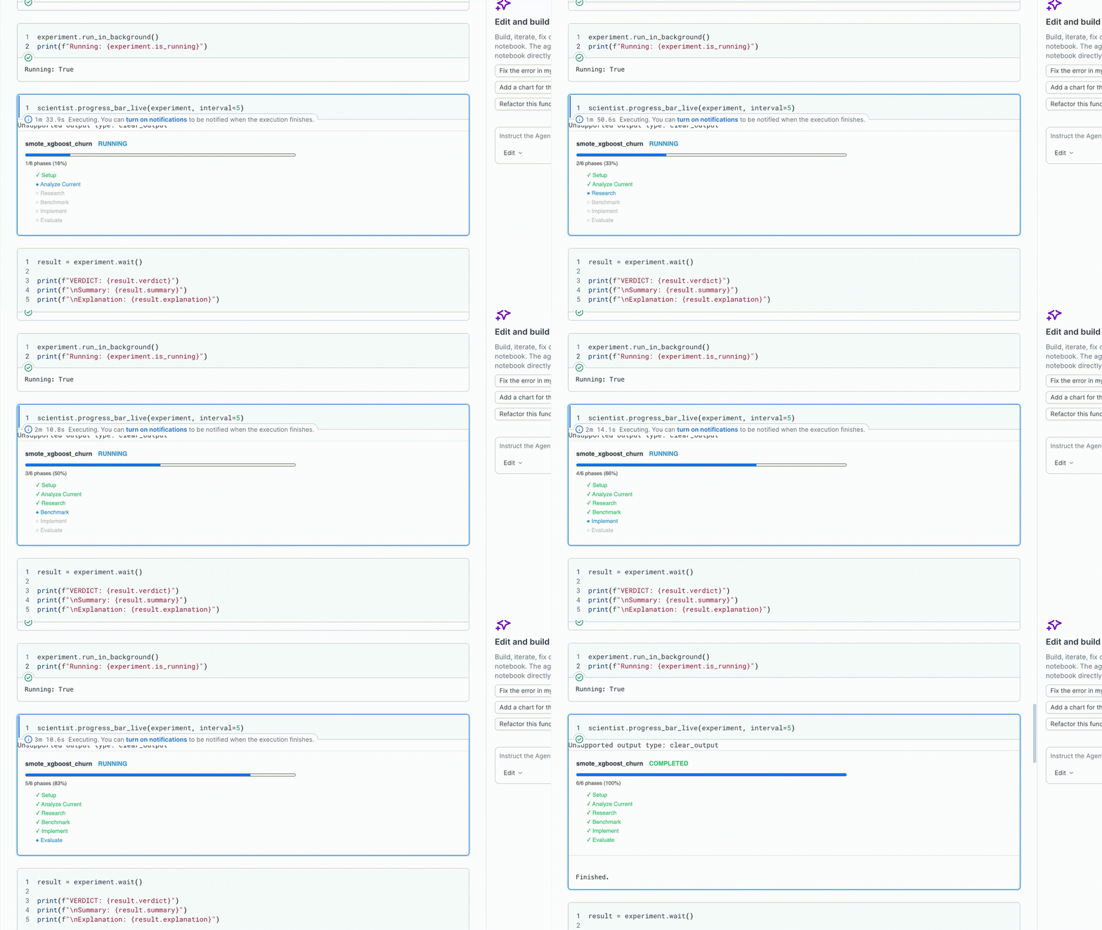 State is exposed on the experiment object at any time:
| Attribute | What it tells you |
| ----------------------- | -------------------------------------------- |
| `experiment.is_running` | `True` while the thread is alive |
| `experiment.is_done` | `True` once finished (success or error) |
| `experiment.error` | The exception if the run raised, else `None` |
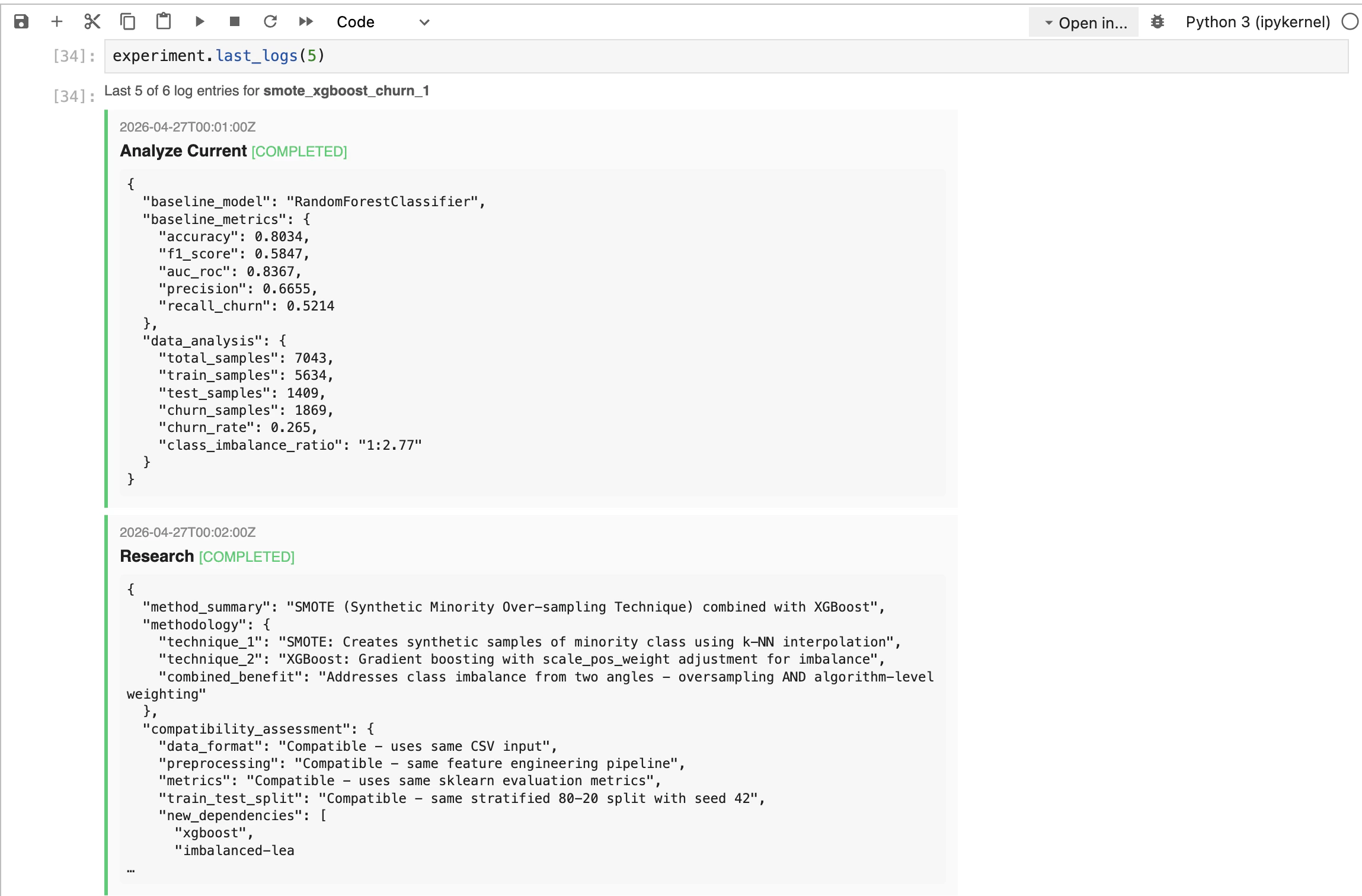
To see the last few things the agent actually did:
```python theme={null}
experiment.last_logs(5)
```
State is exposed on the experiment object at any time:
| Attribute | What it tells you |
| ----------------------- | -------------------------------------------- |
| `experiment.is_running` | `True` while the thread is alive |
| `experiment.is_done` | `True` once finished (success or error) |
| `experiment.error` | The exception if the run raised, else `None` |
To see the last few things the agent actually did:
```python theme={null}
experiment.last_logs(5)
```
 Interrupt the kernel to stop watching without cancelling the run. Call `experiment.stop()` to cooperatively cancel.
### 4. Wait for the result
```python theme={null}
result = experiment.wait()
print(f"VERDICT: {result.verdict}")
print(f"\nSummary: {result.summary}")
print(f"\nExplanation: {result.explanation}")
```
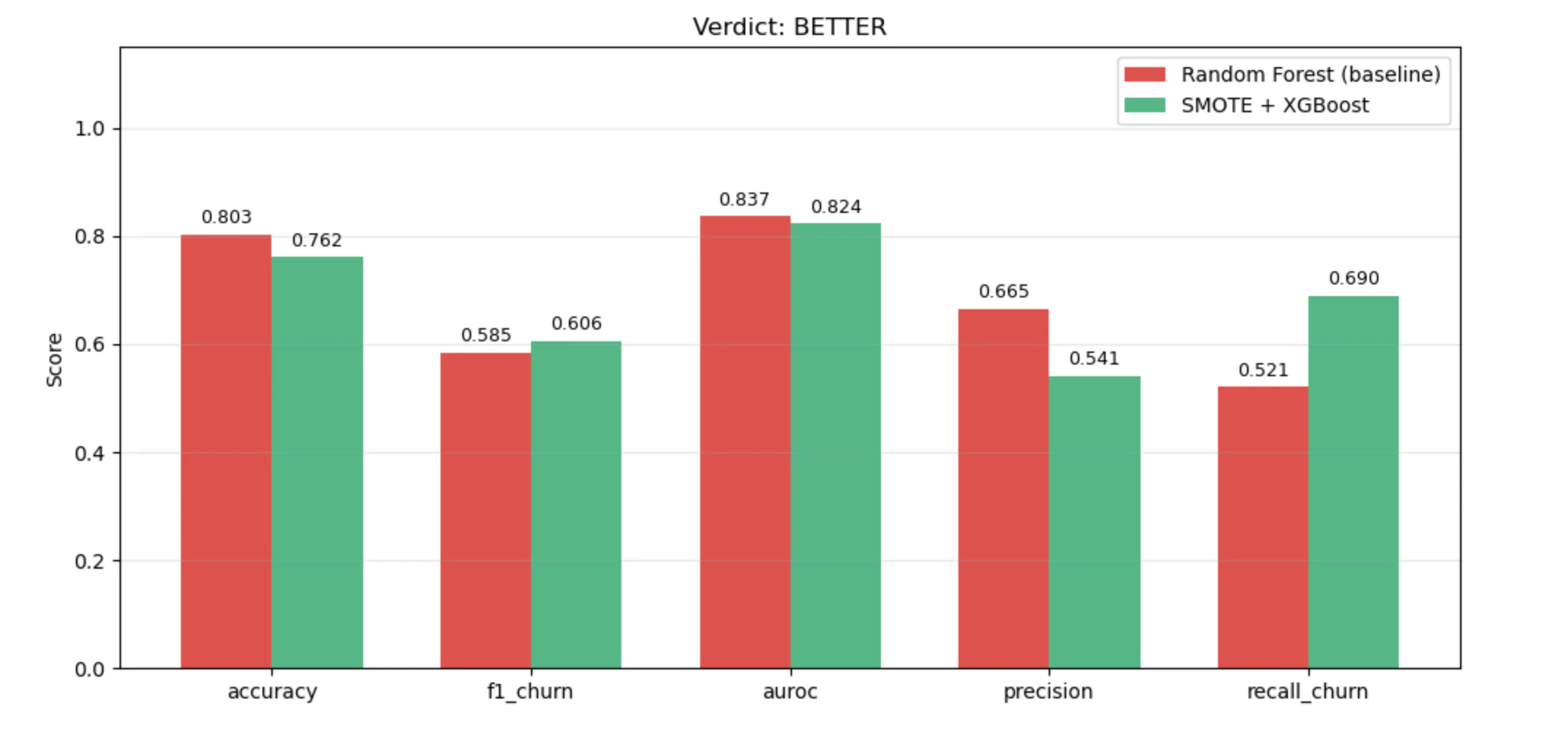
`wait()` blocks until the run finishes and re-raises any exception it produced. For this demo run, it returns:
```text theme={null}
VERDICT: BETTER
Summary: XGBoost combined with SMOTE oversampling significantly improves minority class
detection in churn prediction. While overall accuracy decreases slightly (70.4% vs 80.3%),
the model achieves substantially higher recall for churned customers (85.6% vs 52.1%),
successfully catching more customers at risk of leaving. The F1 score improved from 0.5847
to 0.6055, indicating better balanced performance on the minority class. This trade-off is
favorable for churn prediction where identifying at-risk customers for retention campaigns
is more valuable than overall accuracy.
Explanation: The verdict is BETTER because: (1) Recall improved by +32.2 percentage points
(0.5214 → 0.8556), catching 85.6% of churners vs. only 52.1% before, reducing missed
opportunities for retention by ~60%. (2) F1-score improved by +3.5% (0.5847 → 0.6055),
showing better minority class balance. (3) While accuracy dropped 10.1 percentage points
(expected with SMOTE), the business impact is positive: preventing customer churn is more
valuable than reducing false positives. (4) SMOTE successfully balanced the 2.77:1 class
imbalance to 1:1, and XGBoost's gradient boosting effectively learned improved decision
boundaries.
```
| Attribute | Value |
| -------------------- | ----------------------------------------------------------- |
| `result.verdict` | `'BETTER'` \| `'WORSE'` \| `'INCONCLUSIVE'` \| `'FAILED'` |
| `result.summary` | What the new method is and how it differs from the baseline |
| `result.explanation` | Why this verdict was reached, referencing concrete numbers |
### 5. Inspect the comparison
`result.table` is a list of metric dicts. Drop it into a DataFrame to see the side-by-side:
```python theme={null}
import pandas as pd
pd.DataFrame(result.table)
```
Interrupt the kernel to stop watching without cancelling the run. Call `experiment.stop()` to cooperatively cancel.
### 4. Wait for the result
```python theme={null}
result = experiment.wait()
print(f"VERDICT: {result.verdict}")
print(f"\nSummary: {result.summary}")
print(f"\nExplanation: {result.explanation}")
```
`wait()` blocks until the run finishes and re-raises any exception it produced. For this demo run, it returns:
```text theme={null}
VERDICT: BETTER
Summary: XGBoost combined with SMOTE oversampling significantly improves minority class
detection in churn prediction. While overall accuracy decreases slightly (70.4% vs 80.3%),
the model achieves substantially higher recall for churned customers (85.6% vs 52.1%),
successfully catching more customers at risk of leaving. The F1 score improved from 0.5847
to 0.6055, indicating better balanced performance on the minority class. This trade-off is
favorable for churn prediction where identifying at-risk customers for retention campaigns
is more valuable than overall accuracy.
Explanation: The verdict is BETTER because: (1) Recall improved by +32.2 percentage points
(0.5214 → 0.8556), catching 85.6% of churners vs. only 52.1% before, reducing missed
opportunities for retention by ~60%. (2) F1-score improved by +3.5% (0.5847 → 0.6055),
showing better minority class balance. (3) While accuracy dropped 10.1 percentage points
(expected with SMOTE), the business impact is positive: preventing customer churn is more
valuable than reducing false positives. (4) SMOTE successfully balanced the 2.77:1 class
imbalance to 1:1, and XGBoost's gradient boosting effectively learned improved decision
boundaries.
```
| Attribute | Value |
| -------------------- | ----------------------------------------------------------- |
| `result.verdict` | `'BETTER'` \| `'WORSE'` \| `'INCONCLUSIVE'` \| `'FAILED'` |
| `result.summary` | What the new method is and how it differs from the baseline |
| `result.explanation` | Why this verdict was reached, referencing concrete numbers |
### 5. Inspect the comparison
`result.table` is a list of metric dicts. Drop it into a DataFrame to see the side-by-side:
```python theme={null}
import pandas as pd
pd.DataFrame(result.table)
```
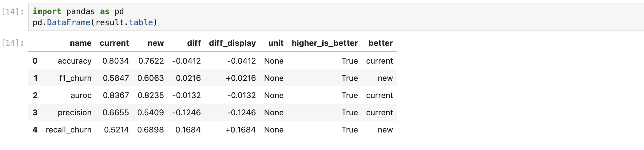 Each row contains:
| Field | Meaning |
| ----------------------- | -------------------------------------------------- |
| `name` | Metric name (e.g. `accuracy`, `f1`, `auroc`) |
| `current` / `new` | Baseline and new-method values |
| `diff` / `diff_display` | Raw difference and a human-friendly version |
| `unit` | Unit of the metric |
| `higher_is_better` | Whether larger is better |
| `better` | Which side won on this metric (`current` or `new`) |
Plotting the table makes the trade-off obvious — in this run, the new method trades a little overall accuracy for a large gain in churn recall:
Each row contains:
| Field | Meaning |
| ----------------------- | -------------------------------------------------- |
| `name` | Metric name (e.g. `accuracy`, `f1`, `auroc`) |
| `current` / `new` | Baseline and new-method values |
| `diff` / `diff_display` | Raw difference and a human-friendly version |
| `unit` | Unit of the metric |
| `higher_is_better` | Whether larger is better |
| `better` | Which side won on this metric (`current` or `new`) |
Plotting the table makes the trade-off obvious — in this run, the new method trades a little overall accuracy for a large gain in churn recall:
 Need the raw artifacts? `result.record` exposes `log.json`, `progress.json`, and registry metadata for the run.
## Managing Experiments
Every experiment is recorded in `experiments.json`. The registry is re-read from disk on every call, so it always reflects current state.
```python theme={null}
scientist.list_experiments() # newest first
scientist.list_experiments(status="completed") # 'in_progress' | 'completed' | 'failed'
exp = scientist.experiments["smote_xgboost_churn"]
exp.phases # normalised phase list
exp.log # parsed log.json
```
Need the raw artifacts? `result.record` exposes `log.json`, `progress.json`, and registry metadata for the run.
## Managing Experiments
Every experiment is recorded in `experiments.json`. The registry is re-read from disk on every call, so it always reflects current state.
```python theme={null}
scientist.list_experiments() # newest first
scientist.list_experiments(status="completed") # 'in_progress' | 'completed' | 'failed'
exp = scientist.experiments["smote_xgboost_churn"]
exp.phases # normalised phase list
exp.log # parsed log.json
```
 Each registry entry is a dict with `name`, `date`, `status`, `verdict`, `baseline_model`, `new_method`, `paper`, and `path`.
## API Reference
```python theme={null}
from upsonic.prebuilt import AppliedScientist
scientist = AppliedScientist(model=..., workspace="./ws")
# Create an experiment
exp = scientist.new_experiment(
"smote_xgboost_churn",
research_source=..., # PDF, URL, repo, Kaggle page, or free-form idea
current_notebook=...,
# current_data=..., # optional
# experiments_directory="./experiments" # optional
)
# Run control
exp.run_in_background()
exp.is_running
exp.is_done
exp.error
exp.stop()
exp.wait() # blocks, returns ExperimentResult
# Progress
exp.progress_bar
scientist.progress_bar_live(exp, interval=5)
exp.last_logs(5)
# Result
res = exp.result
res.verdict # 'BETTER' | 'WORSE' | 'INCONCLUSIVE' | 'FAILED'
res.summary
res.explanation
res.table # list[dict]
# Registry
scientist.list_experiments()
scientist.experiments["smote_xgboost_churn"].phases
scientist.experiments["smote_xgboost_churn"].log
```
The full demo notebook for this agent lives in the Upsonic repo under [prebuilt\_autonomous\_agents](https://github.com/Upsonic/Upsonic/tree/master/prebuilt_autonomous_agents).
Each registry entry is a dict with `name`, `date`, `status`, `verdict`, `baseline_model`, `new_method`, `paper`, and `path`.
## API Reference
```python theme={null}
from upsonic.prebuilt import AppliedScientist
scientist = AppliedScientist(model=..., workspace="./ws")
# Create an experiment
exp = scientist.new_experiment(
"smote_xgboost_churn",
research_source=..., # PDF, URL, repo, Kaggle page, or free-form idea
current_notebook=...,
# current_data=..., # optional
# experiments_directory="./experiments" # optional
)
# Run control
exp.run_in_background()
exp.is_running
exp.is_done
exp.error
exp.stop()
exp.wait() # blocks, returns ExperimentResult
# Progress
exp.progress_bar
scientist.progress_bar_live(exp, interval=5)
exp.last_logs(5)
# Result
res = exp.result
res.verdict # 'BETTER' | 'WORSE' | 'INCONCLUSIVE' | 'FAILED'
res.summary
res.explanation
res.table # list[dict]
# Registry
scientist.list_experiments()
scientist.experiments["smote_xgboost_churn"].phases
scientist.experiments["smote_xgboost_churn"].log
```
The full demo notebook for this agent lives in the Upsonic repo under [prebuilt\_autonomous\_agents](https://github.com/Upsonic/Upsonic/tree/master/prebuilt_autonomous_agents).